Note: this writeup describes work I did with Dr. Garret Kenyon during an SULI internship at Los Alamos National Laboratory in 2010

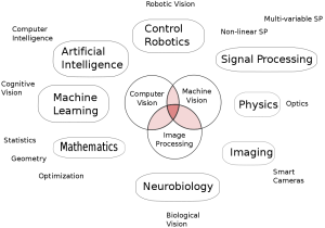
There are many divergent approaches to computer vision. As of yet, no generally accepted approach exists. Figure 1 shows the diverse fields that overlap with computer vision research. Because of the many difficulties of computer vision and absence of a general approach, most research has gone into systems for specialized applications. Much of this research has been successful, for instance we now have algorithms for fingerprint recognition, facial recognition and the classification of simple geometric objects. But we do not have a system which can look at everyday scenes and find objects.

The first approaches to computer vision were highly geometrical in nature. For instance, an algorithm might begin by isolating the edges of the image using various filters, convolutions and spatial derivatives. Next the computer will build a map of these edges and attempt to isolate the boundaries of various objects. In some cases the computer may try to classify vertices (where edges meet) as convex or concave. Next the computer will search a database of pre-programmed object information to find the nearest match. Accomplishing this search may involve mathematical techniques such as tree-search algorithms or gradient decent. Such an algorithm might be able to successfully detect the orientation of simple geometric objects such as cubes or pyramids based on the way the vertices are arranged. The distance and orientation of objects could be calculated using a combination of stereo vision and/or projective geometry. However, such a system would probably fail with curved objects.

While these “geometric” approaches have proven to be fruitful, they have also proven to be quite limited. For this reason, many people are turning to biologically inspired approaches as a solution to the general problem of computer vision.  Originally, computer models of the visual cortex were developed to test the current theories about its function. When they were used for object recognition they were found to outperform all the other approaches in certain cases.

Biological vision

A “biologically-inspired” approach is essentially a reverse engineering of the primate vision system. For this reason it is worth describing briefly what is known about the primate/human vision system. Vision involves much more than “taking a picture”. Focusing and detection of light is just the first stage in a complex system which allows humans to construct a mental picture of the environment. Very much like the pixels on a digital camera, the human eye contains thousands of rods of cones which detect light. However, even on the retina itself, pixel data starts to be encoded for processing. Rods and cones are wired together with amacrine, bipolar, horizontal and ganglion cells to create receptive fields that, loosely speaking, are sensitive to small points of light and edges.

These signals then travel to the Lateral Geniculate Body (LGB), a part of the visual cortex located in the back of the brain. There, signals pass through several layers, known as V1, V2, V3, V4, and V5 (MT). Each of these layers is a complex neural network containing tens of millions of neurons. Altogether there are roughly 150 million neurons in the LGB in humans. In these neural networks there are numerous feedforward and feedback connections between the layers and lateral connections within each layer. At each stage, more sophisticated and abstract processing takes place. For instance, neurons in V1 called “complex cells” are able to detect edge orientation, lines and direction of motion. This abstracted information is sent to higher layers for more processing. Loosely speaking, cells in V3 and V5 help distinguish local and global motion, while cells in V4 appear to be selective of spatial frequency, orientation and color. Other cells coordinate stereo vision. In MT, 2D boundaries of objects might be detected. Figuring out each of these processing steps and mapping the web of connections between the layers is still a nascent field of research.

After processing in the LGB, visual data moves into the Inferior Temporal Gyrus (IT), the temporal lobe, prefrontal cortex and the rest of the brain. Although our understanding of IT is quite poor, it is believed that this region is responsible for mapping a class (such as “car”, “tree”, “pencil”) to parts of the visual data. It appears that some class neurons are very general (“human face”) while other class neurons are more specific (“mother’s face”). There is probably extensive feedback between IT and the lower layers to check different object hypotheses. Such feedback systems would also be essential for learning. Eye movements are directed by the brain to get a better idea what objects are. Some of the larger eye movements are made consciously but the vast majorities are actually unconscious. These eye movements are a very useful area to study but are not relevant to this research since we will be processing still images with a computer.

A paper by Yamane, Carlson et al. entitled “A neural code for three-dimensional object shape in macaque inferotemporal cortex” hypothesizes that certain neurons or collections of neurons in IT are responsible for detecting 3D surface patches. They confirmed this by subjecting macaque monkeys to a variety of shape stimuli and finding the stimuli that gave the best response for neurons. This finding is significant to this research because it means it implies that biological brains analyze surface patches in addition to edges.

“Class descriptions” in the higher brain must be very abstract to facilitate the many different ways an object may appear. For instance, the same object can appear to be large or small and can be viewed from many different orientations. This ability may have to be learned anew for each object or the brain may be able to visualize how an object will appear from different angles on its own. Most likely, there is a mix of both techniques. Object recognition is further complicated by variations in lighting, coloration and other objects (occlusions) that may be in the way. Currently, computer vision systems are very likely to fail when any of these variations are present. Biologically inspired computer vision provides an avenue to overcome such limitations.

Biologically inspired computer vision

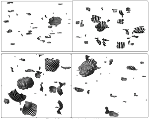
The ultimate goal of this project is build a neural network which can detect various shapes. The first part of the project was to develop a test called the “3D Amoeba task”. This test can be used to compare the computer’s performance with humans. In the test, an image is flashed to the viewer for a very short amount of time. The objective is to say whether there is an “amoeba” present, or whether there is just “debris”. An “amoeba” is a random, lumpy closed 3D shape. “Debris” are pieces that may be lumpy but are not closed – they are flakes. Debris are scattered uniformly throughout space and may occlude the Amoeba. In this project a program was written to create 3D amoebas using random combinations of spherical harmonics, which are basis functions in 3D space. 

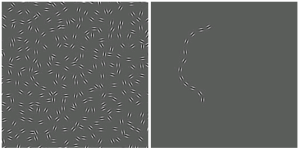
This project builds off a facet of the Petavision project, which simulated the visual cortex using the Roadrunner super computer. Initial experiments simulated 100,000 neurons, and this number was later increased to one million. It was able to complete the “2D Amoeba task”, which was to isolate a wiggly 2D figure amongst debris.

A similar task can be found in a paper by Field, et al. published in 1993 (see figure 2).

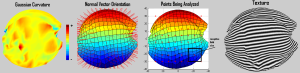
Next, we started to make the kernel, which will store information about surface patches. An amoeba is created and analyzed. There are eight pieces of data to store : x position, y position, Gaussian curvature, two normal vector components, spatial frequency and orientation. The normal vector components are encoded as two angles, theta and phi, measured with respect to the direction of sight. This is simpler then storing them as (x,y,z) components and more intuitive as well.

The program is run many times for many different Amoeba surfaces until a large body of data is collected. This data can then be mapped onto an eight-dimensional array of “neurons”. Each neuron has a Gaussian response curve for each parameter. So, for each patch of an amoeba, the array of neurons is “lit up” in a certain way.  These arrays can be used to train a neural network. Essentially, the neural network learns how to associate given stimuli with curvature and normal vector orientation, which it can’t detect directly. Ultimately it will be able predict the general characteristics of nearby surface patches, assuming the object is closed and smooth. In this way it will be able to detect amoebas since they are always closed and smooth, while debris have discontinuities along their edges.

In conclusion, this project resulted in a program to create a “kernel” of data for training a neural network. This is the first step in the larger project of creating a neural network to detect amoebas. Eventually it is hoped a similar methodology could be used to detect and distinguish arbitrary smooth closed shapes.