Quantum effects in water
Note: although I personally found writing this post to be a useful exercise, unfortunately it turned out to be a rather long, rambling and at times rather technical brain dump. There are enough topics mentioned here for dozens of future posts (not to suggest that I could write on all of the topics mentioned off the top of my head – most would require research on my part.) Likely certain things will be fleshed out in future posts. I would appreciate any feedback if there are particular things my readers would like to see in future posts.
In my last post I made the rather vague statement that quantum effects account for “about 10%” of the properties of water. I was basing this off the well-established understanding that the hydrogen bond is roughly 10% quantum covalent and 90% electrostatic.
Still, no doubt some of my readers may be confused about what I mean by a “quantum effect”. In this post I hope to clarify the term and some of the confusions surrounding the classical / quantum distinction. I will also give some precise examples of quantum effects in water.
First I’d like to get over a possible semantic / philosophical stumbling block, which is the fact that everything is quantum mechanical. This is true. But the world can also be described by classical theory to a large degree of accuracy. Thus the world contains both classical and quantum effects, the former being describable in terms of classical theory to the accuracy required, and the later being describable only in terms of quantum theory to the accuracy required. Usually the classical regime is described as the regime with large masses and big energies – things like baseballs, pendulums and billard balls — this much is obvious. What we are interested in here is knowing to what extent we can understand molecular dynamics and hence, the properties of materials, just by doing classical mechanics (+ some additional low-computational-cost tricks), which is a difficult question. This is a very important question though, from a practical perspective, because quantum mechanical calculations are extremely expensive to perform [roughly speaking, the number of coordinates in a wavefunction grows exponentially with the number of particles.] Only two particles can be solved exactly using quantum mechanics. Using perturbation theory in theory larger ensembles can be solved, using things which look like “Feynman diagrams” in the expansion of the partition function, but in practice this has only proved doable for simple systems like the Leonard-Jones gas — anything more complicated being intractable with current methods. Using variational techniques ground state energies of large systems can be solved to large accuracy, but quantum dynamics in particular remains extremely expensive. Many levels of approximation are needed (Born–Oppenheimer approximation + DFT + Pseudopotentials) to do a quantum dynamics simulation, and even then they are limited to a few hundred atoms and run times of < 100 ps, even on cluster computers.[By comparison, the time it takes a protein to fold ranges from 100,000 ps for fast small ones to several seconds (1s = 1,000,000,000,000 ps) for the larger ones.] Also, calculations of the compressibility and dielectric spectra require simulations of at least a few nanoseconds to hundreds of nanoseconds at low temperatures (1ns = 1000ps). Thus there is a great interest in building molecular models (in particular, of water) which run using classical mechanics (+ additional tricks to capture some of the quantum effects). Besides these practical issues, the aforementioned problem is also interesting from from a pure physics perspective as well, (ie answering it gives us a deeper understanding of nature) as we will see, because we learn more about how classical mechanics ’emerges’ from quantum mechanics. In particular water is known to be a highly quantum mechanical molecule, because it has two hydrogens which play a big role (their low mass => more quantum effects), whereas in large bio molecules people usually don’t care so much about the quantum mechanical nature of the hydrogens.
By a “classical calculation” I mean that we are just integrating (solving) Newton’s second law with some pairwise potential. [non pairwise potentials, such as those which are functions of three bodies, (the famous example being the Axilrod-Teller potential) are known to be important in water, and can be included in classical simulations, but are a huge headache to code, according to the literature. I’ve never seen it done in any publications.] The pairwise potentials that are used are the 1/r Coulomb potential + the Leonard Jones potential and possibly intra molecular potentials, which range considerably in sophistication. On top of this you can also add polarizability , which takes into account the rapid shifting of the electron clouds during each timestep of the simulation. (There are several ways of doing this. In one case you imbed a polarizable dipole in each molecule and then find the equilibrium orientations of all the dipoles at each timestep, which requires solving a large matrix equation. It is not a pairwise interaction, rather it is a cooperative interaction.) In the TTM3 model charge clouds and dipole ‘clouds’ are used to simulate the delocalization of the charge. This takes into account a ”quantum effect” via the classical trick of using a charge cloud to represent the electron wavefuction.
In summary here is a breakdown of the ‘levels of simulation’ , with numbers giving the relative computational cost
- Rigid (“ball and stick”) = 1
- Flexible (“ball and spring”) = 5
- Rigid + Polarizable = 6
- Flexible + Polarizable = 30
- Flexible + Nuclear quantum effects (NQE) = 175
- Classical rigid nuclei + electronic quantum effects via density functional theory (DFT)= 1000
- flexible classical nuclei + DFT = 5000
- DFT + flexible nuclei + NQE = 175000
[This is taken from (Vega, 2011)] What this shows us is that a simulation that takes an hour with a rigid model will take roughly 175,000 hours with a full quantum (also called “ab initio”) simulation. I consider numbers 1-4 to be ‘classical techniques’ whereas 5-8 are quantum techniques.
In classes on quantum mechanics, we are often told that quantum theory reduces to classical theory when “hbar goes to zero”. (hbar being the constant giving defining the energy scale for quantum mechanics, or more precisely, the angular momentum scale, since it has units of angular momentum) This is a rather sloppy statement, because in fact hbar is a constant, as every physicist knows. It is only when the energy scale that we are dealing with become much larger than hbar that – somehow – classical mechanics starts to work. To people working with the path integral formulation of quantum mechanics (which includes both particle theorists and also people doing path-integral molecular dynamics), the classical – quantum transition is seemingly easy to understand, because the path integral formulation transitions perfectly into the famous variational formulation of classical mechanics in the limit that E(x)/hbar » 1 , where E(x) can be either the kinetic or potential energy of the system. This way of thinking isn’t very useful for us – except in so far as the path integral molecular dynamics, which is a technique which helps take into account the nuclear quantum effects in molecular dynamics.
As with everything in life and in physics, subtleties abound. Here I would like to describe several quantum effects which are present in water and ice.
The increase in the dielectric constant upon freezing
Observe the following, from a paper by Abascal & Vega (J. Phys. Chem. A, 2011) (pdf)
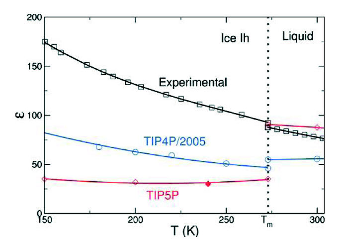 The blue and pink lines show the prediction of two classical models (both of which are among the very best “ball and stick models” yet devised). As you can see , they are quite a bit different from the experimental result. The first difference is in the magnitude. In particular, TIP4P/2005 underestimates the dielectric constant of water. This can be corrected by artificially increasing the dipole moment,(somebody actually did this, I can dig up the reference if anyone wants) but this no doubt compromises other aspects of the model, which is fit to produce many things, the dielectric constant being just one, often of lower priority. The second thing is that the slope (change in dielectric constant with temperature) is different – although this isn’t exactly true in the liquid regime, if you look at more data on TIP4P/2005 you will see that TIP4P/2005 captures the slope in the liquid regime pretty well (indeed, better than other popular ball and stick models). (All of the simulation points have error bars, which unfortunately are not shown here)
The difference which I want to focus on here is the fact that dielectric constant of water increases when going from the liquid to the solid phase, whereas the dielectric constant of the classical models decreases. This is rather peculiar if you think about it. The dielectric constant measures how much polarization you get in a substance when you apply an external electric field. In water, which is dipolar, most of the polarization comes from reorientation of the intrinsic electric dipoles. In most dipolar substances, the dielectric constant decreases upon freezing — when the dipoles become ‘frozen’ in place, they are harder to reorient. But in water, it’s the other way around. As was discovered in the 80s, the reason for this is that in ice there is a new contribution to the polarization, which is the tunneling of protons. This tunneling manifests itself in both the increase in dielectric constant and in a surprisingly high conductivity in ice. During the past few decades this tunneling has been a subject of intense research within the field of ice physics. It is a decidedly quantum effect since nobody has figured out a way to incorporate it into classical simulations.
Anomalous proton diffusion in water – the Grotthuss mechanism
Proton tunneling can also occur in water, although to a lesser extent than in ice, so it doesn’t contribute much to the dielectric constant. (At least, this is what I’ve inferred from the literature. I should run the numbers on this using the experimental data on proton conductivity to see how small the contribution is). However, it leads to an anomalously high diffusion constant for protons in water. (which is a very important effect since whenever you make an acid, you end up with a ton of protons diffusing around). Amusingly, this “quantum effect” was theorized in 1806 by Theodor Grotthuss, although at that time he thought the water molecule was OH and not HOH. Here’s a nice animation of the process from Wikipedia:
 There is no easy way to take this into account something like this in a classical molecular dynamics simulation of acid and water.
The effects of the nuclear quantum effects
As I mentioned earlier, the light hydrogens are a source of many quantum effects in water. The DeBroglie wavelength of a proton with the ‘thermal energy’ at room temperature (kT ~ .025 eV) is about 1.8 angstroms. The width of a hydrogen atom is about 1 angstrom, so this gives some indication that the delocalization of the proton is going to be important. One way to take this into account is to use Path Integral Molecular Dynamics (PIMD). I’m not going to go into PIMD in any detail, but it’s all based on a single mathematical formula called the Trotter expansion:
Exp(A + B) = lim_{P -> infinity} [ Exp[A/(2P)] * Exp[B/P] * Exp[A/(2P)] ]^P
Where A and B are operators (not numbers) in the Hilbert Space. It turns out that using this formula, one can show there is an isomorphism between solution of the quantum mechanical path integral and the solution of a classical system of masses coupled by springs such that they form a circle. “P” corresponds to the number of masses and is also called the “Trotter number” or “number of beads”. In a recent paper by a recent graduate of our group, Sriram Ganeshan , he looks at the oxygen-oxygen radial distribution function (RDF) using PIMD:
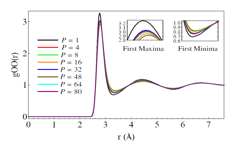 For those of you who don’t know what a radial distribution function is, it shows the average density of atoms a given distance away from a certain atom, compared to the average density those atoms in the entire substance, which is taken as 1. In other words, if you were to be an oxygen atom , it shows what distances you are most likely to see the other oxygen atoms around you. In a solid, the RDF has many peaks which are evenly spaced. In the liquid, the peaks decrease in amplitude. In other words, the solid has long range ordering, whereas the liquid only has short range ordering.
Here you see the difference between a model (TIP4P/2005-F) with the PIMD nuclear quantum effects and without. The difference looks small, but in fact, it’s considered quite large by people who look at these things all the time. What you see is that the maxima are less high and the minima are less low when PIMD is used. This indicates that the quantum effects lead to less structure in the liquid. This makes perfect sense since the protons are ‘delocalized’ , or in other words ‘smeared out’ over space. [In his paper, Ganeshan also studies a method of incorporating these delocalized effects and zero-point effects using what is called ‘colored noise’.]
It would be unfair of me not to mention at this juncture the work of current group member Betül Pamuk on nuclear quantum effects in ice. In ice the zero-point motions of the hydrogens lead to a larger than expected volume at low temperatures. Surprisingly, in heavy water (D20) there is an even larger excess volume, which is really unexpected, because the heavier deuterium should be less quantum than hydrogen. This bizarre effect was first analyzed by our group and explained using some theory. It was experimentally confirmed by Stony Brook University Prof. Peter Stephens using x-ray diffraction, where they also explored what happens when you replace the Oxygen-16 with Oxygen-18. The resulting paper can be found on the ArXiV
The absorption spectrum
This is something which I don’t really understand very well right now, so I won’t attempt to offer a real explanation. However, I would like to show the striking results of several simulations. Here is the infrared absorption spectrum reported by Paesani, Iuchi, and Voth in 2007 (annotated by myself):
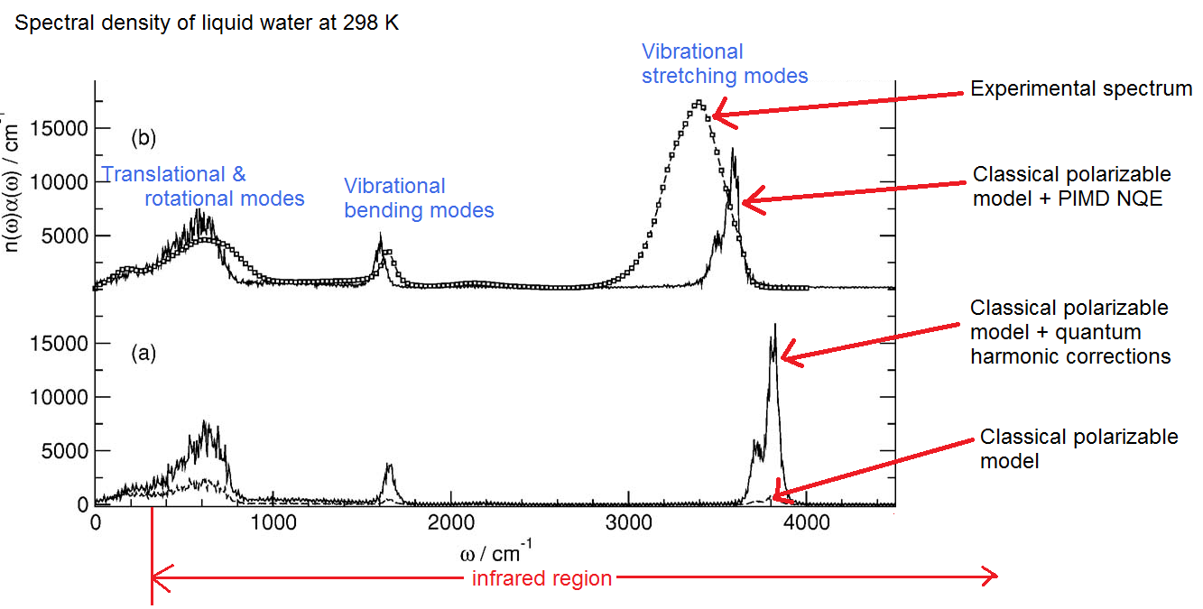 Note the big difference in the classical vs quantum models. The classical model here is a polarizable model called TTM2.1-F which features a very sophisticated treatment of the polarizability. The amplitude of the absorption is much lower in the classical model, and whereas with the NQE the peaks are higher and slightly more ‘smeared out”. The stretching modes of the quantum models (neither of which are ‘full quantum’, taking into full consideration the quantum nuclei and electrons) don’t compare well with experiment, so obviously some quantum effects are not being taken into account.