A physicist’s visualization of Bayes’ theorem
Have you noticed that everyone is talking about Bayes’ theorem nowadays?
Bayes’ theorem itself is not very complicated. The human mind, however, is extremely bad at trying to gain an intuitive understanding of Bayes’ theorem based (Bayesian) reasoning. The counter-intuitive nature of Bayesian reasoning, combined with the jargon and intellectual baggage that usually accompanies descriptions of Bayes’ theorem, can make it difficult to wrap one’s mind around. I am a very visual thinker, therefore, I quickly came up with a visualization of the theorem. A little Googling shows that there are many different ways of visualizing Bayes’ theorem. A few months ago I came across a visualization of Bayes’ theorem which I found somewhat perplexing. Even though mathematical truths are universal, they are internalized differently by every individual. I would love to hear whether others find my visualization approach useful. It is a very physicist-oriented visualization.
Derivation of Bayes’ theorem, with visualization
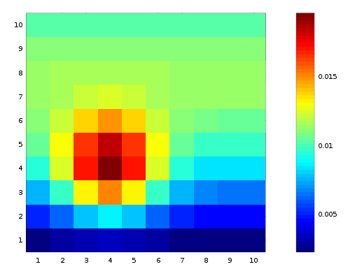
The derivation of Bayes’ theorem rests on the definition of conditional probability. Let’s consider some random variables, X and Y. Capital letters denote random variables, and lowercase denote particular values they may have._ _The joint probability is a function \(P(x,y)\) might look like on our space of possible values:
 ](http://www.moreisdifferent.com/wp-content/uploads/2015/11/plot.png)
This is simply a histogram, normalized so that the sum of all the bins equals 1. Now we ask the following question: given that I have \(y=3\) defines what in physics-speak we would call a “subspace”:
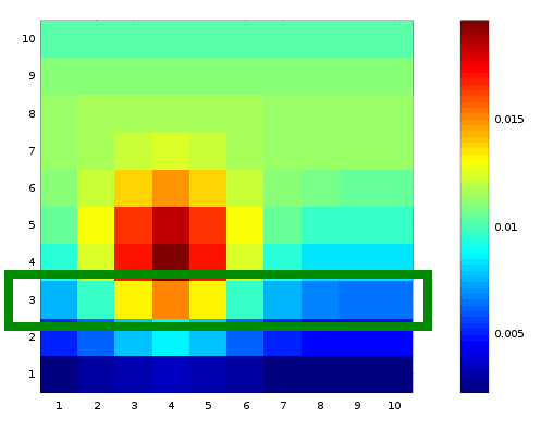
The conditional probability \(P(x,y)\) by normalizing our subspace so that the sum of all the elements in the subspace equals 1. This is done by dividing by
\(\sum_{i=1}^{10} P(x=i, y=3) = P(y=3)\)
Thus, in general the conditional probability is:
\(P(x|y) = \frac{P(x,y)}{P(y)} =\frac{P(x,y)}{\sum_{i=1}^{N}P(i,y)}\)
In the lingo of statisticians, our normalization factor \(y=3\) subspace”.
Based on the equation for conditional probability, we make the following observation:
\(P(y|x) P(y) = P(x,y) = P(x|y) P(x)\)
Dividing the left and right hand sides of this identity by P(y) yields Bayes’ theorem:
\(P(y|x) = \frac{ P(x|y) P(x) }{ P(y) }\)
Example
The archetypical example of applying Bayes’ theorem is (stolen from MacKay’s book):
Jo has a test for a nasty disease. We denote Jo’s state of health by the variable a and the test result by b.
if a = 1 Jo has the disease
if a = 0 Jo does not have the disease.
__The result of the test is either positive’ (b = 1) or negative’ (b = 0); the test is 95% reliable: in 95% of cases of people who really have the disease, a positive result is returned, and in 95% of cases of people who do not have the disease, a negative result is obtained. The final piece of background information is that 1% of people of Jo’s age and background have the disease. Jo has the test, and the result is positive. What is the probability that Jo has the disease?
To solve this problem we first note that \(\quad\quad =.059\)
We plug these things into Bayes’ theorem:
\(\quad\quad = .16\)
So, despite the positive result on the test, the probability he actually has the disease is only .16, or 16%. Our intuition often fails us with such problems, because we neglect to notice that the base rate of the disease is very small (1%). If the base rate is on the same order of magnitude as how often the test gives a false positive, then a positive result on a test won’t be able to tell us whether a patient has a disease with very much certainty.
An inference problem
Now let’s consider a classic inference problem. There are 10 different urns, each with 10 balls. Urn \(u\)?
The conditional probability of drawing \(u\)is :
\[P(n_B|u, N) =\binom{N}{n_B} \left(\frac{u}{10}\right)^{n_B} \left(1-\frac{u}{10}\right)^{N-n_B}\]Prior to drawing any balls, we assume each urn is equally likely, so \(P(u) = 1/10\)(yes, this is an assumption. in the words of MacKay, “you can’t do inference without making assumptions”). The conditional probability and prior probability allow us to construct the joint probability:
\[P(u, n_B) = P(n_B | u) P(u)\]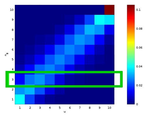
The joint probability contains all the information we need. We simply consider the subspace \(n_B = 3\)(highlighted in the figure above) and properly normalize it. The normalization factor is :
\[P(n_B = 3) = \sum_{i=1,10} P(u=i, 3)=0.0957\]This process amounts to plugging the above quantities into Bayes’ theorem:
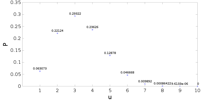
\[P(u | n_B = 3) = \frac{P(n_B=3 | u) P(u)}{P(n_B = 3)}\]The result is :
Jargon
Because of its importance, there is a lot of jargon attached to Bayes’ theorem. Once you learn the jargon, reading stats articles becomes a lot easier!
**evidence – **this is whatever we measured so far.
**hypothesis – **the model we are testing
likelihood – the likelihood tells us, given hypothesis/model x, what the probability of the evidence we observed? People can get rather semantic here. MacKay says “never say ‘likelihood of the data’.. always say ‘likelihood of the parameters’. The likelihood function is not a probability distribution. ”
prior – the term prior refers to our ‘prior’ knowledge. In many cases, our prior knowledge is zero, so we give each possibility an equal probability. For instance, in the case of the urns, since there were 10 possible urns, we assigned each a prior probability of 1/10. The prior is where different general assumptions can be made.
marginal – in physics language, we would call this the ‘normalization factor’ or the probability of being in the subspace determined by the evidence/measurements.
Further reading:
_Information Theory, Inference, and Learning Algorithms _David J. Mackay (free to read online)