DIY Drug Discovery - using molecular fingerprints and machine learning for solubility prediction
Warning: unfortunately since this post was imported from Wordpress, the code may contain formatting errors! Sorry!
This is going to be the first in a series of posts on what I am calling “DIY Drug Discovery”. Admittedly, though, this title is hyperbolic. Discovering a new drug requires bringing it through a series of trials, which is very hard, if not impossible for an individual to do themselves. What I’m really going to be discussing is DIY drug screening. I believe in the near future individuals will be able to discover candidate drug molecules using commodity GPU hardware and open source software, such as scikit-learn.org, https://keras.io/, http://www.rdkit.org/ and https://deepchem.io/.
Table of contents
- Background on chemical space and drug discovery
- Basic concepts of fingerprinting
- Testing out different machine learning models
- Conclusion
- Addendum : solubility datasets
Background on chemical space and drug discovery
The set of all possible molecules, which is known as chemical space, is incredibly vast. The Chemical Abstracts Service (CAS) registry lists 49,037,297 known molecules (molecules that have actually be synthesized). The number of different molecules that have been synthesized, in both public and private settings, may reach towards 100,000,000. Yet this is only tiny fraction of the number of possible molecules. Recent research has tried to enumerate the number of possible molecules containing Carbon, Nitrogen, Oxygen, Hydrogen, Oxygen, and halogens which may be of interest for drug discovery. So far, possible molecules up to a size of 17 atoms have been enumerated and a large database called GBD has been created. Enumerating possible molecules isn’t as simple as enumerating possible molecular graphs. There are many physical constraints that the authors had to take into account. For instance:
-
bonding - many types of bonds are not possible – covalent bonds must be between an electron donor and an electron acceptor. A Chlorine atom cannot bond to a flourine and a sodium cannot bond to a magnesium.
-
geometrical constraints - Due to the nature of atomic orbitals, each atom prefers to bond in particular configuration. For instance, carbon prefers to bond tetrahedrally and when forming rings prefers to form hexagons. Pentagons and other shapes are not necessarily impossible, but they are generally high unstable. For instance, cubane, where carbon is forced to bond at 90 degrees, is highly unstable and explosive material. Carbon bonding in a triangle, or an isolated pentagon or decagon is impossible.
-
functional group stability - Many arrangements may be structurally stable in isolation but are highly reactive, making them near impossible to contain in the real world. For instance, if an oxygen or nitrogen atom is bonded to a non-aromatic C=C, this creates an Enol or enamine group which is highly reactive. The authors of the GBD database used 12 seperate filters to limit what types of functional groups could exist.
-
stereochemistry - the basic idea of this constraint is that “two things cannot be in the same place at the same time”. For instance, a molecule cannot loop back and intersect itself.
-
synthesizability - the molecule most be synthesizable. For instance molecules with more than three carbon rings or allenes (C=C=C) are exceedingly difficult to synthesize.
These basic physical constraints reduce the size of the chemical space significantly. For instance the authors of GBD note “The vast majority of fused small ring systems are high strained and reactive. 96.7% of molecules with carbon are removed by this constraint. However, even after applying 29 filters, the GBD database still contains 10^11 molecules. This is a large number, but tractable in the sense that it could be stored on the very latest computer hardware. (storing the database in SMILES format would consume about 63 terabytes. The entire database is not available for public consumption, only a subset of 50 million compounds is downloadable). Keep in mind that this number was obtained after applying many constraints - the number of organic molecules of drug like size with normal atoms (CNOH + halogens) and up to 4 rings has been estimated to be around 10^60!
Apart from whether a molecule can physically exist and be synthesized, there are further constraints when it comes to making a drug:
-
solubility the molecule must be soluble in the blood.
-
toxicity the molecule cannot be toxic.
-
permeability & lipophilicity can it get through any biological membranes it needs to, such cell wall or the blood brain barrier?
-
binding target affinity will it actually bind to the target of interest?
Traditionally drug design has been done through a trial and error approach. A professor once described it to me as “trying to build an airplane by attaching the wings in at random orientations, and then seeing if it flies.” Just as computer simulations are used to design highly aerodynamic airplanes, so that less actual physical assembly and testing needs to be done, physics based simulation holds the promise of being able to design and optimize drug molecules before they are actually syntheized.
However quantum simulations are extremely computationally intensive and approximate methods often are not accurate enough, so would be very helpful if machine learning could be used to screen molecules instead.
Basic concepts of fingerprinting
For more info an in easy to read format, see the http://www.daylight.com/dayhtml/doc/theory/theory.finger.html.
The first step in molecular machine learning is encoding the structure of the molecule in a form that is amenable to machine learning. This is where a lot of research is currently focused. A useful representation encodes features that are relevant and is efficient, so as to avoid the curse of dimensionality. Fortunately, there is a way method of featurazation called fingerprinting which already has a long history of development in the world of drug discovery.
Fingerprinting was originally designed to solve the problem of molecular substructure search – how do I find all the molecules in my database with a particular substructure? A related problem is molecular similarity - given a molecule, how do I find the molecules in my database that are most similar. Only later were fingerprints applied for machine learning, or what has traditionally called quantitative structure property relationships (QSPR).
Fingerprinting creates an efficient representation of the molecular graph. The basic process of fingerprinting is as follows: First the algorithm generates a set of patterns. For instance, enumeration of different paths is common:
| 0-bond paths: | 1-bond paths: |
| C | OC |
| O | C==C |
| N | CN |
| 2-bond paths: | 3-bond paths: |
| OC=C | OC=CN |
| C=CN |
Storing all this data would result in an enormous representation. The trick of fingerprinting is to “hash” each of these features, which essentially means they act as seeds to a random number generator called a hash function. The hash function generates a bit string. Typically the hash function is chosen so that 4 or 5 bits per pattern are non-zero in the bit string. Next, all of the bit strings are OR’ed together.
This process is very useful for substructure searching because every bit of the substructure’s fingerprint will be on (=1) in the molecule’s fingerprint. Accidental collisions between patterns or substructures are possible, but if the bit density is low (known as a sparse representation) they are rare. Ideally, the on bit density of the bitstring should be tuned so as to reach a particular discriminatory power that is needed (ie. the chance that two structurally different molecules in my database have the same fingerprint is only 1%). There is a tradeoff between discriminatory power and the efficiency of the representation.
In practice, creating a bit density is done through folding. A very long, very sparse fingerprint is ‘folded’ down (with OR operations) to create a fingerprint with a desired length and good bit density. In case this is not obvious what this means, it can be literally thought of as folding the vector onto itself.
Now let’s test some fingerprints. We use rdkit.org, an open source cheminformatics library. Our data consists of https://en.wikipedia.org/wiki/Simplified_molecular-input_line-entry_system strings, which encode molecular graphs into a string of characters, and experimentally determined solubility values.
from rdkit import Chem
from rdkit.Chem.EState import Fingerprinter
from rdkit.Chem import Descriptors
from rdkit.Chem.rdmolops import RDKFingerprint
import pandas as pd
import numpy as np
from sklearn.preprocessing import StandardScaler
from sklearn import cross_validation
from keras import regularizers
from keras.models import Sequential
from keras.layers import Dense, Activation, Dropout
from sklearn import cross_validation
from sklearn.kernel_ridge import KernelRidge
from sklearn.linear_model import Ridge, LinearRegression
from sklearn.svm import SVR
from sklearn.neighbors import KNeighborsRegressor
from sklearn.gaussian_process import GaussianProcessRegressor
from sklearn.neural_network import MLPRegressor
from sklearn.ensemble import GradientBoostingRegressor, RandomForestRegressor
from sklearn.model_selection import GridSearchCV
from rdkit.Avalon.pyAvalonTools import GetAvalonFP

#Read the data
data = pd.read_table('../other_data_sets/solubility_data.txt', sep=' ', skipfooter=0)

def estate_fingerprint_and_mw(mol):
    return np.append(FingerprintMol(mol)[0], Descriptors.MolWt(x))

#Add some new columns
data['Mol'] = data['SMILES'].apply(Chem.MolFromSmiles)
num_mols = len(data)

#Create X and y
#Convert to Numpy arrays
y = data['Solubility'].values
from rdkit.Chem.rdMolDescriptors import
from rdkit.Chem.AtomPairs.Sheridan import GetBPFingerprint
from rdkit.Chem.EState.Fingerprinter import FingerprintMol
from rdkit.Avalon.pyAvalonTools import GetAvalonFP #GetAvalonCountFP  #int vector version
from rdkit.Chem.AllChem import  GetMorganFingerprintAsBitVect, GetErGFingerprint
from rdkit.DataStructs.cDataStructs import ConvertToNumpyArray
import rdkit.DataStructs.cDataStructs

def ExplicitBitVect_to_NumpyArray(bitvector):
    bitstring = bitvector.ToBitString()
    intmap = map(int, bitstring)
    return np.array(list(intmap))


class fingerprint():
    def __init__(self, fp_fun, name):
        self.fp_fun = fp_fun
        self.name = name
        self.x = []

    def apply_fp(self, mols):
        for mol in mols:
            fp = self.fp_fun(mol)
            if isinstance(fp, tuple):
                fp = np.array(list(fp[0]))
            if isinstance(fp, rdkit.DataStructs.cDataStructs.ExplicitBitVect):
                fp = ExplicitBitVect_to_NumpyArray(fp)
            if isinstance(fp,rdkit.DataStructs.cDataStructs.IntSparseIntVect):
                fp = np.array(list(fp))

            self.x += [fp]

            if (str(type(self.x[0])) != "<class 'numpy.ndarray'>"):
                print("WARNING: type for ", self.name, "is ", type(self.x[0]))

def make_fingerprints(length = 512, verbose=False):
    fp_list = [
         #fingerprint(lambda x : GetBPFingerprint(x, fpfn=AtomPair),
         #            "Physiochemical properties (1996)"), ##NOTE: takes a long time to compute
         fingerprint(lambda x : GetHashedAtomPairFingerprintAsBitVect(x, nBits = length),
                     &qfuot;Atom pair (1985)"),
         fingerprint(lambda x : GetHashedTopologicalTorsionFingerprintAsBitVect(x, nBits = length),
                     "Topological torsion (1987)"),
         fingerprint(lambda x : GetMorganFingerprintAsBitVect(x, 2, nBits = length),
                     "Morgan circular "),
         fingerprint(FingerprintMol, "Estate (1995)"),
         fingerprint(lambda x: GetAvalonFP(x, nBits=length),
                    "Avalon bit based (2006)"),
         fingerprint(lambda x: np.append(GetAvalonFP(x, nBits=length), Descriptors.MolWt(x)),
                    "Avalon+mol. weight"),
         fingerprint(lambda x: GetErGFingerprint(x), "ErG fingerprint (2006)"),
         fingerprint(lambda x : RDKFingerprint(x, fpSize=length),
                     "RDKit fingerprint")
    ]

    for fp in fp_list:
        if (verbose): print("doing", fp.name)
        fp.apply_fp(list(data['Mol']))

    return fp_list

fp_list = make_fingerprints()
def test_model_cv(model, x, y, cv=20):
    scores = cross_validation.cross_val_score(model, x, y, cv=cv, n_jobs=-1,
scoring='neg_mean_absolute_error')

    scores = -1scores

    return scores.mean()


def test_fingerprints(fp_list, model, y, verbose = True):

    fingerprint_scores = {}

    for fp in fp_list:
        if verbose: print("doing ", fp.name)
        fingerprint_scores[fp.name] = test_model_cv(model, fp.x, y)

    sorted_names = sorted(fingerprint_scores, key=fingerprint_scores.__getitem__, reverse=False)

    print("\\begin{tabular}{c c}")
    print("           name        &  avg abs error in CV (kJ/cc) \\\\")
    print("\\hline")
    for i in range(len(sorted_names)):
        name = sorted_names[i]
        print("%30s & %5.3f \\\\" % (name, fingerprint_scores[name]))
    print("\\end{tabular}")


test_fingerprints(fp_list, Ridge(alpha=1e-9), y, verbose=True)
def test_model_cv(model, x, y, cv=20):
    scores = cross_validation.cross_val_score(model, x, y, cv=cv, n_jobs=-1, scoring='neg_mean_absolute_error')

    scores = -1\*scores

    return scores.mean()


def test_fingerprint_vs_size(model, num_sizes_to_test = 20, max_size=2048, cv = 20, verbose=False, makeplots=False):

    fp_list = make_fingerprints(length = 10) #test
    num_fp = len(fp_list)

    sizes = np.linspace(100,max_size,num_sizes_to_test)

    scores_vs_size = np.zeros([num_fp, num_sizes_to_test])

    num_fp = 0
    for i in range(num_sizes_to_test):
        if verbose: print(i, ",", end='')
        length = sizes[i]
        fp_list = make_fingerprints(length = int(length))
        num_fp = len(fp_list)
        for j in range(num_fp):
            scores_vs_size[j,i] = test_model_cv(model, fp_list[j].x, y)

    if (makeplots):
        import matplotlib.pyplot as plt
        plt.clf()
        fig = plt.figure(figsize=(10,10))
        fp_names = []
        for i in range(num_fp):
            plt.plot(sizes, scores_vs_size[i,:],'-')
            fp_names += [fp_list[i].name]
        plt.title('Ridge regression, average CV score vs fingerprint length',fontsize=25)
        plt.ylabel('average mean absolute error in CV ',fontsize=20)
        plt.xlabel('fingerprint length', fontsize=20)
        plt.legend(fp_names,fontsize=15)
        plt.ylim([.2,4])
        plt.show()

    return scores_vs_size


scores_vs_size = test_fingerprint_vs_size(Ridge(alpha=1e-9), verbose=True, makeplots=True)

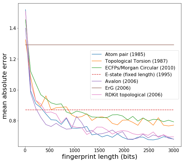
Now we see expected behaviour -- fingerprint performance increases as the length is increased, and eventually converges around 2000 bits. Note that the Estate has a fixed length of 80 and is more like a descriptor set rather than a fingerprint. Another point is that Lasso regression (L1 regularization) generally does slightly better than Ridge regression with fingerprints, since fingerprints can have elements which are always zero or almost always zero. [L1 regularization introduces a penalty term which has a gradient that forces coefficients corresponding to variables with no predictive power to be precisely zero, whereas L2 has trouble getting coefficients to be precisely zero.] In what follows, I use the Estate fingerprint, as I was comparing Estate with some other applications. I create a new data matrix *X* and then feed into machine learning models:
def estate_fingerprint(mol):
    return FingerprintMol(mol)[0]

#Scale X to unit variance and zero mean
data['Fingerprint'] = data['Mol'].apply(estate_fingerprint)

X = np.array(list(data['Fingerprint']))

st = StandardScaler()
X = np.array(list(data['Fingerprint']))
X = st.fit_transform(X)
KRmodel = GridSearchCV(KernelRidge(), cv=10,
              param_grid={"alpha": np.logspace(-10, -5, 10),
             "gamma": np.logspace(-12, -9, 10), "kernel" : ['laplacian', 'rbf']}, scoring='neg_mean_absolute_error', n_jobs=-1)

KRmodel = KRmodel.fit(X, y)
Best_KernelRidge = KRmodel.best_estimator_
print("Best Kernel Ridge model")
print(KRmodel.best_params_)
print(-1*KRmodel.best_score_)
Rmodel = GridSearchCV(Ridge(), cv=20,
              param_grid={"alpha": np.logspace(-10, -5, 30),}, scoring='neg_mean_absolute_error', n_jobs=-1)

Rmodel = Rmodel.fit(X, y)
Best_Ridge = Rmodel.best_estimator_
print("Best Ridge model")
print(Rmodel.best_params_)
print(-1*Rmodel.best_score_)
GPmodel = GridSearchCV(GaussianProcessRegressor(normalize_y=True), cv=20,
              param_grid={"alpha": np.logspace(-15, -10, 30),}, scoring='neg_mean_absolute_error', n_jobs=-1)
GPmodel = GPmodel.fit(X, y)
Best_GaussianProcessRegressor = GPmodel.best_estimator_
print("Best Gaussian Process model")
print(GPmodel.best_params_)
print(-1*GPmodel.best_score_)
RFmodel = GridSearchCV(RandomForestRegressor(), cv=20,
              param_grid={"n_estimators": np.linspace(50, 150, 25).astype('int')}, scoring='neg_mean_absolute_error', n_jobs=-1)

RFmodel = RFmodel.fit(X, y)
Best_RandomForestRegressor = RFmodel.best_estimator_
print("Best Random Forest model")
print(RFmodel.best_params_)
print(-1*RFmodel.best_score_)
Testing out different machine learning models
import matplotlib.pyplot as plt
from sklearn.metrics.pairwise import rbf_kernel
def make_scatter_plot(y_pred_train, y_pred_test, y_train, y_test, title='', figsize=(6,4), fontsize=16):
plt.clf()
plt.figure(figsize=figsize)
plt.scatter(y_train,y_pred_train, label = 'Train', c='blue')
plt.title(title,fontsize=fontsize+5)
plt.xlabel('Experimental Solubility (mol/L)', fontsize=fontsize)
plt.ylabel('Predicted Solubility (mol/L)', fontsize=fontsize)
plt.scatter(y_test,y_pred_test,c='lightgreen', label='Test', alpha = 0.8)
plt.legend(loc=4)
plt.show()
def test_models_and_plot(x, y, model_dict, plots=True):
''' test a bunch of models and print out a sorted list of CV accuracies
inputs:
x: training data features, numpy array or Pandas dataframe
y: training data labels, numpy array or Pandas dataframe
model_dict: a dictionary of the form {name : model()}, where 'name' is a string
and 'model()' is a scikit-learn model object.
'''
mean_scores = {}
percent_errors = {}
for (name, model) in model_dict.items():
#print("running %s" % name)
scores = cross_validation.cross_val_score(model, x, y, cv=20, n_jobs=-1, scoring='neg_mean_absolute_error')
scores = -1*scores
mean_score = scores.mean()
mean_scores[name] = mean_score
X_train, X_test, y_train, y_test = cross_validation.train_test_split(x, y, test_size=0.1)
model.fit(X_train, y_train)
y_pred_train = model.predict(X_train)
y_pred_test = model.predict(X_test)
percent_error = np.mean( 100*np.abs(y_test -y_pred_test)/np.abs(y_pred_test))
percent_errors[name] = percent_error
fulltitle = name+'\n mean % error: '+str(percent_error)
if plots:
make_scatter_plot(y_pred_train, y_pred_test, y_train, y_test, title=fulltitle, figsize = (8,6))
sorted_names = sorted(percent_errors, key=mean_scores.__getitem__, reverse=False)
print("\\begin{tabular}{c c c}")
print(" name & % test err & . abs error in CV \\\\ ")
print("\\hline")
for i in range(len(sorted_names)):
name = sorted_names[i]
print("%30s & %5.3f & %5.3f \\\\" % (name, percent_errors[name], mean_scores[name]))
print("\\end{tabular}")
alpha_grid = {'alpha': np.logspace(1e-11,1e-1,8)}
model_dict = {
'Linear Regression': LinearRegression(),
'Kernel Ridge Regression': Best_KernelRidge,
'Ridge Regression':Best_Ridge,
'Guassian Process Regressor': Best_GaussianProcessRegressor,
'Support Vector Regression': SVR(),
'KNeighborsRegressor': KNeighborsRegressor(),
'Neural Network': MLPRegressor(alpha=100,max_iter=8000, hidden_layer_sizes=[8,6], early_stopping=False),
'Gradient Boosted Trees': GradientBoostingRegressor(n_estimators=100),
'Random forest': Best_RandomForestRegressor
}
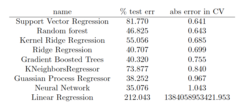
test_models_and_plot(X, y, model_dict)


The output is formatted in LaTeX so a nice table can be produced, which ends up looking like this:
Conclusion
The best performing model in this case was support vector regression, followed closely by Random Forrest and Kernel Ridge Regression. In general, I find that KRR and random forest are usually the best performing models, and this is the first time SVR has won out. However, in molecular machine learning, the model that is used is really not the limiting factor, provided one does their due diligence and explores several classes of models and optimizes their hyperparameters. The component which really determines success is the featurization technique used. The machine learning model can be thought of an black box machine that extracts the nonlinear dependence of Y on X. As long as the black box is large enough and very well tuned and regularized, we don’t have to worry about it much. What we need to worry about more is creating the right X from our molecule data so that the black box can do its job. Traditionally, human created fingerprints and descriptors have been used, which are based on physics and chemical intuition about what molecular features are important. In the future ML can also be applied to fingerprint design – this will be discussed in a future post.
Another thing we observe is the large difference between the test and CV errors. The test error is for a particular train-test split, and appears to have high variance. The CV error is averaged over all test-train splits. The percentage error depends highly on whether one is working with a very soluble or insoluble molecule. For some applications the error profile of this model may be acceptable, in others it may be too crude. The error is definitely larger than a different application I applied this same code to, which was predicting decomposition energy. In that case I obtained average errors on the order of ~20% or less.
Addendum : solubility datasets
It was requested that I include the solubility datasets. Here they are, along with the original papers:
Delaney_paper.pdf
delaney_solubility_data_1129_mols.csv
description_of_Huuskonen_molecules.pdf
Huuskonen_paper.pdf
Huuskonen_README.md
Huuskonen_solubility_data_1311_mols.csv
solubility_combined_2291_mols.csv
If you use any of these data, please cite the original papers.